Introduction to Gravitational lensing

Einstein predicted that light should get deflected in the presence of a massive object using the principle of equivalence. According to the principle of equivalence, a uniform gravitational field is equivalent to an accelerated frame of reference, and no local experiment should be able to distinguish between two such frames.

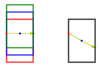
Consider a frame of reference, say an elevator, and a light ray entering this elevator at t=0 through a small hole made at the midpoint of the elevator. If the elevator is at rest in vacuum, the light ray should exit horizontally through another hole dug on the other wall exactly at its midpoint. If the elevator is moving with a velocity \(v\), the vertical coordinate of the elevator would have changed during the time taken by light to cross the width of the elevator. Light still travels in a straight line in this case but the line is not horizontal as seen from the elevator.

import pylab as pl
%pylab inline

conf = %config InlineBackend.rc
conf["figure.figsize"] = (6, 6)
conf['savefig.dpi']=300
conf['font.serif'] = "Computer Modern"
conf['font.sans-serif'] = "Computer Modern"
conf['text.usetex']=True

width = 600
%config InlineBackend.rc
%pylab inline

import matplotlib as mpl
mpl.rcParams['figure.dpi']= 300

Populating the interactive namespace from numpy and matplotlib
Populating the interactive namespace from numpy and matplotlib

import pylab as pl
import matplotlib.patches as patches

def draw_box(x, y, ax, color):
    rect = patches.Rectangle((x, y), 0.3, 0.6, linewidth=5, edgecolor=color, facecolor='none', alpha=0.7)
    # Add the patch to the Axes
    ax.add_patch(rect)

ax = pl.subplot(1, 1, 1)

# Draw boxes
draw_box(0.0, 0.1, ax, "red")
draw_box(0.0, 0.2, ax, "blue")
draw_box(0.0, 0.3, ax, "green")

# Add arrow for the light ray
ax.arrow(0.0, 0.5, 0.27, 0.0, color='y', lw=2, linestyle="--", head_width=0.03, width=0.001)
ax.scatter([0.0], [0.5], color="r")
ax.scatter([0.15], [0.5], color="b")
ax.scatter([0.3], [0.5], color="g")

# Remove axes
ax.set_axis_off()

# Draw boxes
draw_box(0.7, 0.1, ax, "black")

# Add arrow for the light ray
ax.arrow(0.7, 0.5, 0.27, -0.18, color='y', lw=2, linestyle="--", head_width=0.03, width=0.001)
ax.scatter([0.7], [0.5], color="r")
ax.scatter([0.85], [0.4], color="b")
ax.scatter([1.0], [0.3], color="g")

<matplotlib.collections.PathCollection at 0x7f2dc7c9c730>

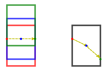
However, if the elevator is accelerating, instead of seeing the light travel in a straight line, a person inside the elevator will observe it to follow a path which curves further downwards. This is because the elevator would have travelled more distance in the vertical direction between the blue and the green points than it did between the red and blue points.

import pylab as pl
import matplotlib.patches as patches

def draw_box(x, y, ax, color):
    rect = patches.Rectangle((x, y), 0.3, 0.6, linewidth=5, edgecolor=color, facecolor='none', alpha=0.7)
    # Add the patch to the Axes
    ax.add_patch(rect)

ax = pl.subplot(1, 1, 1)

# Draw boxes
draw_box(0.0, 0.1, ax, "red")
draw_box(0.0, 0.2, ax, "blue")
draw_box(0.0, 0.4, ax, "green")

# Add arrow for the light ray
ax.arrow(0.0, 0.5, 0.27, 0.0, color='y', lw=2, linestyle="--", head_width=0.03, width=0.001)
ax.scatter([0.0], [0.5], color="r")
ax.scatter([0.15], [0.5], color="b")
ax.scatter([0.3], [0.5], color="g")

# Remove axes
ax.set_axis_off()

# Draw boxes
draw_box(0.7, 0.1, ax, "black")

# Add arrow for the light ray
ax.arrow(0.7, 0.5, 0.27/2, -0.18/2, color='y', lw=2, linestyle="--", head_width=0.03, width=0.001)
ax.arrow(0.7+0.27/2., 0.5-0.18/2, 0.27/2, -0.32/2, color='y', lw=2, linestyle="--", head_width=0.03, width=0.001)

ax.scatter([0.7], [0.5], color="r")
ax.scatter([0.85], [0.4], color="b")
ax.scatter([1.0], [0.2], color="g")

<matplotlib.collections.PathCollection at 0x7f2dc92124d0>

The equivalence principle implies that we should see a similar phenomenon where we observe light to be travelling in an apparent curved path when light is travelling in a gravitational field.

The deflection of light in the weak field limit

In the weak field limit , the distances in spacetime can be measured using the perturbed Minkowski metric given by

\begin{eqnarray} ds^2 = -\left(1+\frac{2\Phi}{c^2}\right) c^2 dt^2 + \left(1-\frac{2\Phi}{c^2}\right) dl^2\,, \end{eqnarray}

where \(\Phi\) is the gravitational potential and \(dl^2\) is the Euclidean metric. Light travels on null geodesics with \(ds^2=0\). This implies that the speed of light, \(c'\) in the presence of such a weak field will be

\begin{eqnarray} c' = \left[\frac{dl^2}{dt^2}\right]^{1/2} = c \left[\frac{\left(1+\frac{2\Phi}{c^2}\right)}{\left(1-\frac{2\Phi}{c^2}\right)} \right]^{1/2} \simeq c \left(1+\frac{2\Phi}{c^2}\right)\,. \end{eqnarray}

Given that the potential will be negative, this implies that the speed of light in the weak field limit will be smaller than the speed of light in vacuum. The second term of this equation is quite small given that we are working in the weak field limit (for point masses, this implies we are working at distances larger than the Schwarzschild radius).

Such a reduction in the speed of light also happens in media with refractive index, \(n\). Rays of light which move between media of different refractive index undergo refraction. Einstein worked out that light rays should similarly get deflected in the presence of a gravitational field. He used the Huygen’s principle to demonstrate this.

He considered a wavefront of light as shown below, and two points separated on the wavefront by separation \(dx\). This separation is perpendicular to the direction of propagation of light. The two points act as separate sources of secondary waves. The speed of light at these two positions however differs due to the different value of the potentials at these locations. This difference is given by \begin{eqnarray} \delta c' &=& (\delta c'/\delta x) \delta x \\ &=& 2 \delta \Phi/(c \delta x) \delta x\,. \end{eqnarray} The new wavefront will be the envelope of the new wavefronts by the corresponding sources. Given the different sizes of the wavefront, the envelope will now travel in a slightly different direction.

In a small time interval \(\delta t\), the difference in the radii of these two circles will be \(\delta c' \delta t\). The deflection angle is the angle made by the common tangent to the two circles with the original wavefront. Here is the picture from Einstein’s 1911 paper on the subject.

\begin{eqnarray} \delta \alpha &=& -\frac{\partial c'}{\partial x} \delta t \\ &=& -\frac{2}{c}\frac{\partial \Phi}{\partial x} \delta t \\ &=& -\frac{2}{c^2}\frac{\partial \Phi}{\partial x} c\delta t \\ &=& -\frac{2}{c^2}\frac{\partial \Phi}{\partial x} \delta l \\ \alpha &=& \int \delta \alpha = -\int \frac{2}{c^2}\nabla_{\perp} \Phi dl \end{eqnarray}

For a point mass one can compute this total deflection angle by using the Born approximation, where the deflection can be calculated and summed over the unperturbed path of the ray. Consider a light ray that travels at a projected distance \(R\) away from a mass \(M\). The potential at any 3-d distance \(r\) from the point mass is given by \begin{eqnarray} \Phi = -\frac{GM}{r} \end{eqnarray}

From the spherical symmetry, it is clear that the deflection has to be in the plane that consists of the point mass and the path of the unperturbed light ray. Let us consider the plane corresponding to the path of the ray and the center of point mass. In this case the perpendicular direction is the \(x-\)direction. Therefore, \begin{eqnarray} \nabla_{\perp} \Phi &=& -\frac{\partial}{\partial x} \frac{GM}{[x^2+y^2]^{1/2}}\\ &=& \frac{GM}{r^2}\frac{\partial r}{\partial x}\\ &=& \frac{GM}{r^2}\frac{x}{r} \end{eqnarray}

If we consider the impact parameter to be \(R\), then \(r=[R^2+y^2]^{1/2}\).

\begin{eqnarray} \alpha &=& \int ds \frac{2}{c^2}\frac{GM}{r^2}\cos \theta \end{eqnarray} Integrating along the path of the unperturbed ray (Born approximation), we get \(ds = dy = R \sec^2 \theta d\theta\) and \(r^2=R^2/\cos^2\theta\), thus, \begin{eqnarray} \alpha &=& \int_{-\pi/2}^{\pi/2} d\theta \frac{2}{c^2}\frac{GM \cos^2\theta}{R^2} R \sec^2\theta \cos \theta \\ &=& \int_{-\pi/2}^{\pi/2} d\theta \frac{2}{c^2}\frac{GM}{R} \cos \theta \\ &=& \frac{4GM}{c^2R} \end{eqnarray}

Plugging in the mass of the Sun and the radius of the Sun, we obtain

\begin{eqnarray} \alpha = \frac{4GM}{c^2R} = 1.75"\left(\frac{M}{M_\odot}\right)\left(\frac{R_\odot}{R}\right) \end{eqnarray}

The deflection is towards the mass and in the plane that we considered above.

This value of the deflection angle as a function of distance from the Sun were confirmed experimentally by Arthur Eddington and colleagues during the solar eclipse in 1919. They observed the positions of stars with respect to the Sun during the Eclipse and compared to the position many months apart when the Sun was not near the stars.

Gravitational lensing by a thin lens

In most astrophysical cases of interest we would be considering a thin lens, where the extent of the lens is much smaller than the distances between the lens and the source or the lens and the observer. An extended lens can be characterized by its surface density in the plane of the sky \(\Sigma(\vec \xi')\).

Consider a small mass element \(\Sigma(\vec \xi') d\vec \xi'\). This small mass element will cause a deflection in its direction. The total deflection for light rays arriving at a position \(\vec \xi\) will be the vector summation of all deflections due to all such mass elements in the plane of the lens.

\begin{eqnarray} \vec {\hat \alpha}(\vec \xi) = \frac{4G}{c^2}\int d^2\vec \xi' \Sigma(\vec \xi') \frac{(\vec\xi-\vec\xi')}{ |\vec\xi-\vec\xi'|^2} \end{eqnarray} where \(D_{\rm d}\) is the angular diameter distance of the lens.

The bold line shows the path of the light ray from a source which is at a true angular position \(\vec \beta\). The light ray eventually reaches the observer on Earth at an angle \(\vec\theta\). The total deflection angle \(\vec {\hat\alpha}\) is the angle between the light ray paths before and after the deflection as shown in the above figure. We also show the angular diameter distance between us and the deflector lens as \(D_{\rm d}\), that between us and the source as \(D_{\rm s}\), and that between the deflector and the source as \(D_{\rm ds}\).

One can define the scaled deflection angle defined to be the angle between the true position of the source and the observed image as shown in the above figure. The scaled deflection angle is given by \begin{eqnarray} \vec \alpha (\vec \theta) = \frac{D_{\rm ds}}{D_{\rm s}} \vec {\hat \alpha}(\vec \theta) \,. \end{eqnarray} From geometry we also obtain the lens equation \begin{eqnarray} \vec \beta = \vec \theta - \vec \alpha (\vec \theta) \,. \end{eqnarray}

Note that here we are using vector signs to denote all angles. This is because the deflection angle from an extended deflector will be a vector not always pointing towards the center of mass of the deflector, and it depends upon the entirety of the mass distribution in the lens plane.

The easiest way to consider this is to consider the above diagram but as seen in the plane of the sky.

The lens equation is a non-linear equation which relates the true position of the source to the observed position of the image as seen by an observer via the deflection angle. Given the mass distribution in the lens plane, and a true source position, one can solve the above equation to obtain the location \(\vec\theta\) where the image will be formed.

Note also that the above equation is non-linear. Although we get one value of the source position \(\vec\beta\) for a given position of the image \(\vec\theta\), we can have multiple values of \(\vec \theta\) for a given true source position.

Point mass deflector

For a point mass deflector the deflection angle was derived by Einstein as we saw above. The lens equation will be given by

\begin{eqnarray} \vec \beta &=& \vec \theta - \frac{D_{\rm ds}}{D_{\rm s}} \frac{4GM}{c^2 D_{\rm d}}\frac{\vec\theta} {|\theta|^2}\\ &=& \vec\theta - \theta_{\rm E}^2\frac{\vec\theta}{|\theta|^2}\,, \end{eqnarray} where we have defined a quantity called \(\theta_{\rm E}\) Due to the spherical symmetry it is clear that \(\vec \theta\) and \(\vec \beta\) will be in the same direction and the lens equation in this case is a one dimensional equation.

\begin{eqnarray} \frac{\beta}{\theta_{\rm E}} &=& \frac{\theta}{\theta_{\rm E}} - \frac{\theta_{\rm E}}{\theta}\,, \end{eqnarray}

Let us make a plot of \(\beta/\theta_{\rm E}\) versus \(\theta/\theta_{\rm E}\).

import pylab as pl
import numpy as np

colors = pl.rcParams['axes.prop_cycle'].by_key()['color']

theta_by_thetaE = np.linspace(0.1, 4.0, 100)
beta_by_thetaE = theta_by_thetaE - 1./theta_by_thetaE
ax = pl.subplot(111)
ax.set_xlim(-5., 5)
ax.set_ylim(-5., 5)
ax.axvline(0.0, color="k")
ax.axhline(0.0, color="k")

ax.plot(theta_by_thetaE, theta_by_thetaE, color="k", linestyle="dashed")
ax.plot(-theta_by_thetaE, -theta_by_thetaE, color="k", linestyle="dashed")

ax.plot(theta_by_thetaE, beta_by_thetaE, color=colors[0])
ax.plot(-theta_by_thetaE, -beta_by_thetaE, color=colors[0])

ax.axhline(0.5, linestyle="-.", color=colors[1])

jk=ax.set_xlabel(r"$\theta/\theta_{\rm E}$")
jk=ax.set_ylabel(r"$\beta/\theta_{\rm E}$")

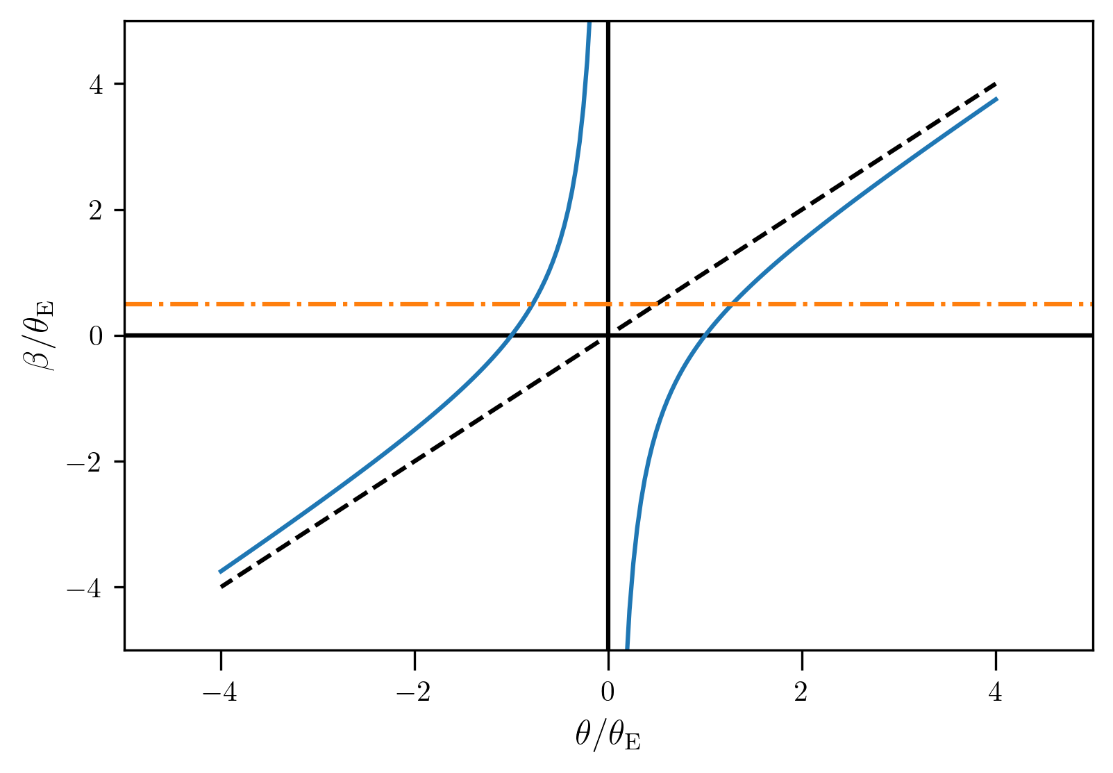
The orange line corresponding to a particular \(\beta\) results in two solutions for \(\theta\) on either side of the lens. \begin{eqnarray} \frac{\theta}{\theta_{\rm E}} = \frac{\beta \pm \sqrt{\beta^2+4\theta_{\rm E}^2}}{2\theta_{\rm E}} \end{eqnarray}

For large values of \(\beta\), in addition to \(\theta \sim \beta\) there is another solution on the other side of the lens with \(\theta\rightarrow 0\). As we will see later such images which form closer to the center are highly demagnified.

For \(\beta=0\), we get two solutions \(\theta=-\theta_{\rm E}\) and \(\theta=\theta_{\rm E}\). In this case however there is no direction to \(\beta\) and instead because of the azimuthal symmetry, images will form on a ring instead of radius \(\theta_{\rm E}\). Such a ring of images is called an Einstein ring and it happens in cases where the alignment of the lens and the source is near perfect, and the lens is very close to spherical symmetry. See an example below of an almost Einstein ring.

The angular separation between the two images will be given by

\begin{eqnarray} \Delta \theta = \sqrt{\beta^2+4\theta_{\rm E}^2} \approx 2\theta_{\rm E} = 2 \left[\frac{4GM}{c^2}\frac{D_{\rm ds}}{D_{\rm d}D_{\rm s}}\right]^{1/2}\,, \end{eqnarray}

and it helps to give a very good estimate of the mass of the point mass deflector if the distances to the lens and source are known in addition to the position of the images.

General thin lens

Let us return back to the case of the general lens. The scaled deflection angle in the lens equation is given by

\begin{eqnarray} \vec \alpha &=& \frac{D_{\rm ds}}{D_{\rm s}} \vec{\hat \alpha}\\ &=& \frac{D_{\rm ds}}{D_{\rm s}} \frac{4G}{c^2}\int d^2\vec \xi' \Sigma(\vec \xi') \frac{(\vec\xi-\vec\xi')}{ |\vec\xi-\vec\xi'|^2} \\ &=& \frac{D_{\rm ds}D_{\rm d}}{D_{\rm s}} \frac{4G}{c^2}\int d^2\vec \theta' \Sigma(\vec \xi') \frac{(\vec\theta-\vec\theta')}{ |\vec\theta-\vec\theta'|^2} \\ &=& \frac{1}{\pi}\int d^2\vec \theta' \frac{\Sigma(\vec \theta')}{\Sigma_{\rm crit}} \frac{(\vec\theta-\vec\theta')}{ |\vec\theta-\vec\theta'|^2} \\ &=& \frac{1}{\pi}\int d^2\vec \theta' \kappa(\vec \theta') \frac{(\vec\theta-\vec\theta')}{ |\vec\theta-\vec\theta'|^2} \end{eqnarray}

where we have defined \(\kappa = \Sigma/\Sigma_{\rm crit}\), and the critical surface density is a geometrical factor which depends upon the lens and source configurations.

\begin{eqnarray} \Sigma_{\rm crit} = \frac{c^2}{4 \pi G}\frac{D_{\rm s}}{D_{\rm d} D_{\rm ds}}\,. \end{eqnarray}

Lensing potential

If we consider the gradient of scalar field \(\ln (|\theta-\theta'|)\) on the two dimensional plane of the sky, we can show that \begin{eqnarray} \nabla_{\vec\theta} \ln (|\vec\theta-\vec\theta'|) = \frac{\vec\theta-\vec\theta'}{|\vec\theta-\vec\theta'|^2} \end{eqnarray}

This implies we can write the scaled deflection angle as the gradient of a potential. \begin{eqnarray} \vec \alpha &=& \frac{1}{\pi}\int d^2\vec \theta' \kappa(\vec \theta') \frac{(\vec\theta-\vec\theta')}{ |\vec\theta-\vec\theta'|^2} \\ &=& \frac{1}{\pi}\int d^2\vec \theta' \kappa(\vec \theta') \nabla_{\vec\theta} \ln (|\vec\theta-\vec\theta'|)\\ &=& \nabla_{\vec\theta} \left[ \frac{1}{\pi}\int d^2\vec \theta' \kappa(\vec \theta') \ln (|\vec\theta-\vec\theta'|)\right]\\ &=& \nabla_{\vec\theta} \psi(\vec\theta) \end{eqnarray} where the potential \(\psi\) is called the lensing potential and is given by \begin{eqnarray} \psi(\vec\theta)&=& \left[ \frac{1}{\pi}\int d^2\vec \theta' \kappa(\vec \theta') \ln (|\vec\theta-\vec\theta'|)\right]\\ \end{eqnarray} It is convenient to work with the lensing potential \(\psi\) since it is a scalar field. If you consider the divergence of the scaled deflection angle we obtain \begin{eqnarray} \nabla.\vec \alpha &=& \frac{1}{\pi}\int d^2\vec \theta' \kappa(\vec \theta') \nabla.\frac{(\vec\theta-\vec\theta')}{ |\vec\theta-\vec\theta'|^2} \\ &=& 2 \int d^2\vec \theta' \kappa(\vec \theta') \delta_{\rm D}(\vec\theta-\vec\theta') \\ &=& 2\kappa\,, \end{eqnarray} and therefore \(\nabla^2\psi = 2\kappa\), where we have used the identity \begin{eqnarray} \delta_{\rm D}(\vec \theta) = \frac{1}{2\pi} \nabla.\frac{\vec\theta}{ |\vec\theta|^2} \end{eqnarray} One can show by explicitly computing the divergence that the right hand side equals zero for \(\theta\neq 0\), and the application of the divergence theorem over a circular area centered at \(\theta=0\) shows that the quantity is a Dirac delta function indeed.

Axially symmetric lenses

For the case of axially symmetric lenses, the scaled deflection angle, \(\vec \alpha\), is expected to be in the direction of \(\theta\). Now consider the integral of \(\vec \alpha.d\vec l\) over a circle at distance \(\theta\). This integral should be equal to \(2\pi\theta\,\alpha\). However, we also have \begin{eqnarray} \oint \vec \alpha.\hat n dl = \int dA \nabla.\vec \alpha = \int dA \nabla^2\psi = \int dA 2 \kappa \end{eqnarray} This will imply \begin{eqnarray} 2\pi\theta\,\alpha = 2 \int dA \Sigma/\Sigma_{\rm crit}\\ \alpha = \frac{1}{\pi \theta\Sigma_{\rm crit}} \int_{0}^{\theta} \Sigma 2 \pi \theta' d\theta' \end{eqnarray} and \begin{eqnarray} \alpha(\theta) = \frac{D_{\rm ds}}{D_{\rm s}} \frac{4GM(<\theta)}{c^2D_{\rm d} \theta} \end{eqnarray}

For beta = 0, \(\alpha=\theta\equiv\theta_{\rm E}\), and thus we obtain \begin{eqnarray} \theta_{\rm E} = \alpha = \frac{D_{\rm ds}}{D_{\rm s}} \frac{4GM(<\theta)}{c^2D_{\rm d} \theta_{\rm E}} \end{eqnarray}

Singular isothermal sphere

Another commonly used deflector model is that of a singular isothermal sphere, where the three dimensional density profile \(\rho(r)\) is given by, \begin{eqnarray} \rho(r) = \frac{\sigma_{\rm v}^2}{2 \pi G r^2} \end{eqnarray} Such models for the three dimensional profiles lead to flat rotation curves because the enclosed mass \(M(<r) \propto r\). The surface density for this model is given by \begin{eqnarray} \Sigma(\xi) &=& \int^{\infty}_{-\infty} \rho([\xi^2+z^2]^{1/2}) dz\\ &=& \frac{\sigma_{\rm v}^2}{2 \pi G \xi}\left[\tan^{-1}\left(\frac{z}{\xi}\right) \right]^{\infty}_{-\infty}\\ &=& \frac{\sigma_{\rm v}^2}{2 G \xi} \end{eqnarray}

We can use the axial symmetry to work out the deflection angle in this case \begin{eqnarray} \alpha(\xi) &=& \frac{1}{\pi \theta\Sigma_{\rm crit}} \int_{0}^{\theta} \frac{\sigma_{\rm v}^2}{G D_{\rm d}\theta'} \pi \theta' d\theta'\\ &=& \frac{1}{\theta \frac{c^2}{4 \pi G}\frac{D_{\rm s}}{D_{\rm d} D_{\rm ds}}} \int_{0}^{\theta} \frac{\sigma_{\rm v}^2}{G D_{\rm d}\theta'} \theta' d\theta'\\ &=& \frac{1}{\theta \frac{c^2}{4 \pi G}\frac{D_{\rm s}}{D_{\rm d} D_{\rm ds}}} \int_{0}^{\theta} \frac{\sigma_{\rm v}^2}{G D_{\rm d}} d\theta'\\ &=& 4\pi\frac{\sigma_{\rm v}^2}{c^2}\frac{D_{\rm ds}}{D_{\rm s}} \end{eqnarray} This implies that the scaled deflection angle is a constant in the case of a singular isothermal sphere.

Consider the lens equation \(\beta = \theta - \alpha(\theta)\). Given that the deflection angle is a constant, it implies that for a source which is perfectly aligned with the lens \(\beta=0\), we will get an Einstein ring at \(\theta_{\rm E}=\alpha\). The Einstein radius in the case of the singular isothermal sphere is \begin{eqnarray} \theta_{\rm E} &=& 4\pi\frac{\sigma_{\rm v}^2}{c^2}\frac{D_{\rm ds}}{D_{\rm s}} \end{eqnarray}

The lens equation is therefore given by \begin{eqnarray} \vec\beta = \vec\theta - \theta_{\rm E} \frac{\vec\theta}{|\theta|} \end{eqnarray}

import pylab as pl
import numpy as np

colors = pl.rcParams['axes.prop_cycle'].by_key()['color']

theta_by_thetaE = np.linspace(0.1, 4.0, 100)
beta_by_thetaE = theta_by_thetaE - 1.
ax = pl.subplot(111)
ax.set_xlim(-3., 3)
ax.set_ylim(-3., 3)
ax.axvline(0.0, color="k")
ax.axhline(0.0, color="k")

ax.plot(theta_by_thetaE, theta_by_thetaE, color="k", linestyle="dashed")
ax.plot(-theta_by_thetaE, -theta_by_thetaE, color="k", linestyle="dashed")

ax.plot(theta_by_thetaE, beta_by_thetaE, color=colors[0])
ax.plot(-theta_by_thetaE, -beta_by_thetaE, color=colors[0])

ax.axhline(0.5, linestyle="-.", color=colors[1])

jk=ax.set_xlabel(r"$\theta/\theta_{\rm E}$")
jk=ax.set_ylabel(r"$\beta/\theta_{\rm E}$")

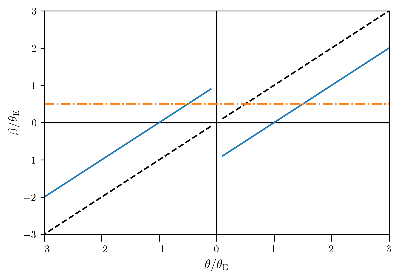
For a singular isothermal sphere this implies that we have only one image if \(|\beta|>\theta_{\rm E}\) and two images when \(\beta<\theta_{\rm E}\). We can also show that the image separation is given by \(2\theta_{\rm E}\).

Magnification matrix

The lens equation transforms locations on the source plane to the locations on the image plane. The magnification of each image is related to the Jacobian of this transformation.

\begin{eqnarray} M(\vec\theta) = |{\cal M}(\vec\theta)| = \left|\frac{\partial\vec\theta}{\partial \vec\beta}\right|_{\vec \theta} \end{eqnarray} The inverse of the magnification matrix is a symmetric 2x2 matrix with components \begin{eqnarray} {\cal M^{-1}}_{ij} = \frac{\partial {\beta_i}}{\partial {\theta_j}} = \delta_{ij} - \frac{\partial \alpha_i}{\partial{\theta_j}} = \delta_{ij} - \frac{\partial^2 \psi}{\partial{\theta_j}\partial \theta_i}\,. \end{eqnarray}

\begin{eqnarray} \mathcal{M}^{-1}(\boldsymbol{\theta}) &=& \begin{pmatrix} 1 - \psi_{11} & -\psi_{12}\\ -\psi_{12} & 1-\psi_{22} \end{pmatrix} \\ \mathcal{M}^{-1}(\boldsymbol{\theta})&=& \begin{pmatrix} 1 - \kappa - \gamma_1 & -\gamma_{2}\\ -\gamma_2 & 1-\kappa + \gamma_1 \end{pmatrix} \\ &=& (1-\kappa)\begin{pmatrix} 1-\frac{\gamma_1}{(1-\kappa)} & -\frac{\gamma_2}{(1-\kappa)} \\ -\frac{\gamma_2}{(1-\kappa)} & 1+\frac{\gamma_1}{(1-\kappa)} \end{pmatrix} \end{eqnarray}

where we have defined a quantity called shear with two components given by \begin{eqnarray} \gamma_1 &=& \frac{1}{2} \left[ \psi_{,11} - \psi_{,22} \right] \\ \gamma_2 &=& \psi_{,12} \end{eqnarray} The inverse magnification matrix shows that the total effect of gravitational lensing on the image of a source can be separated into two effects: one magnifies the image uniformly in all directions by a factor \(1-\kappa\), and the second effect leads to a shear on top of it. One can further define \begin{eqnarray} {\boldsymbol \gamma} &=& \gamma_1 + i \gamma_2=|{\boldsymbol \gamma}|e^{i2\phi} \end{eqnarray}

One can perform a diagonalization of the above magnification matrix to find the eigenvalues and eigenvectors in which the image of a galaxy gets sheared. \begin{eqnarray} |\mathcal{M}^{-1}-\lambda I|&=& \left|\begin{pmatrix} 1 - \kappa - \gamma_1 - \lambda & -\gamma_{2}\\ -\gamma_2 & 1-\kappa + \gamma_1 - \lambda \end{pmatrix}\right| = 0 \\ 0&=& (1-\kappa-\lambda)^2-\gamma_1^2-\gamma_2^2]\\ \lambda &=& 1 - \kappa \pm |\gamma| \end{eqnarray} A circular image of a source with radius \(R\) gets distorted to an elliptical image with axes \begin{eqnarray} \frac{R}{1-\kappa-|{\boldsymbol \gamma}|}; \frac{R}{1-\kappa+|{\boldsymbol \gamma}|}\,. \end{eqnarray}

To understand the relation between the definition of the phase \(\phi\) in the shear, consider that the larger eigenvector is inclined at an angle \(\phi\) with respect to the x-axis. In this case, we get, \begin{eqnarray} \begin{pmatrix} 1 - \kappa - \gamma_1 & -\gamma_{2}\\ -\gamma_2 & 1-\kappa + \gamma_1 \end{pmatrix} \begin{pmatrix} 1\\ \tan\phi \end{pmatrix} = (1-\kappa+\gamma) \begin{pmatrix} 1\\ \tan\phi \end{pmatrix} \end{eqnarray} which implies \begin{eqnarray} (1-\kappa-\gamma_1) -\gamma_2 \tan \phi &=& 1 -\kappa + |\gamma| \,.\\ \tan \phi = -\frac{|\gamma|+\gamma_1}{\gamma_2} \end{eqnarray} Using \begin{eqnarray} \tan 2\phi = \frac{2\tan\phi}{1-\tan^2\phi}, \end{eqnarray} we obtain \begin{eqnarray} \tan 2\phi = \frac{\gamma_2}{\gamma_1}\,. \end{eqnarray}

A circular source thus gets distorted in to an ellipse, where the angle of orientation is related the relative ratio of the two shear components, and the difference in the axis is related to the shear at the location of the source.

Note that the two eigenvalues can have either the same signs or opposite signs, which leads to images of either same or opposite parities. Accordingly images are divided in to different types. Type I images have

The magnification is therefore given by \begin{eqnarray} M = |{\cal M}| = \frac{1}{(1-\kappa+|\gamma|)(1-\kappa-|\gamma|)} \end{eqnarray} At locations where any of the terms in the denominators approach zero, the magnification become formally infinite. Such locations in the image plane are called critical curves, and correspond to images with large magnifications such as arcs. The corresponding regions in the source plane are called caustics.

The caustics divide the source plane into regions with different multiplicity. The number of images changes as the source crosses a caustic. The figure below from Ellis (2010) shows the caustics and the critical curves for a singular isothermal ellipsoid lens.

Depending upon the sign of the eigenvalues you can have different types of images. Type I images have both positive eigenvalues. Type II images have opposite signs for the two eigenvalues. Type III images on the other hand have both negative eigenvalues. Type I and III have positive parity which means they have same parity as the original source. Type II images on the other hand have negative parity.

Time delays between images

Consider the quantity \begin{eqnarray} \tau (\vec\theta; \vec\beta) = \frac{1}{2}\left( \vec\theta - \vec\beta \right)^2 - \psi(\vec\theta) \end{eqnarray}

Equating the gradient of \(\tau\) with respect to \(\theta\) to zero gives the lens equation \begin{eqnarray} \nabla \tau (\vec\theta; \vec\beta) &=& \vec\theta - \vec\beta - \nabla\psi(\vec\theta) \\ 0 &=& \vec\theta - \vec\beta -\vec\alpha \end{eqnarray}

The quantity \(\tau\) is called the Fermat potential. The Fermat potential for a given value of \(\beta\) represents the time of arrival of image at a given location \(\theta\). Images form at the stationary points of the Fermat potential surface. The first term in the Fermat potential corresponds to the path difference between the unperturbed path and the perturbed path, while the second term is a result of the gravitational time delay induced on the path of light ray due to the presence of the deflector.

The actual time delay between the unperturbed path of the light ray and the perturbed path of the ray is given by \begin{eqnarray} T(\vec\theta; \vec\beta) = (1+z_{\rm d})\frac{D_{\rm d}D_{\rm s}}{D_{\rm ds}c}\tau (\vec\theta; \vec\beta) \end{eqnarray} upto a numerical additive constant potential.

In order to derive the above expression, let us first consider the geometric time delay due to the light path.

Consider OUA and SUC be isosceles triangles. In this case the geometric path difference between the red unperturbed light path and the perturbed path is given by the sum of lengths AB and BC. From geometry, angles OUA and OAU should be equal to \(90-(\theta-\beta)/2\). Similarly angles SUC and SCU should be equal to \(90-\gamma/2\) where we denote the angle USC to be \(\gamma\). The angle AUC is therefore equal to \((\theta-\beta+\gamma)/2=\hat\alpha/2\). This implies that the path length difference is equal to UB\(\hat\alpha/2\). The length UB is equal \(D_{\rm d}(\theta-\beta)\), while \(\hat\alpha=\alpha \frac{D_{\rm s}}{D_{\rm ds}}\). The path length difference is thus equal to \begin{eqnarray} \Delta L &=& \frac{1}{2}D_{\rm d}(\theta-\beta) \alpha \frac{D_{\rm s}}{D_{\rm ds}}\\ &=& \frac{1}{2}(\theta-\beta)^2 \frac{D_{\rm d} D_{\rm s}}{D_{\rm ds}} \end{eqnarray} The time delay introduced due to this term will be equal to \((1+z_{\rm d})\Delta L/c\) purely due to geometrical effect, \begin{eqnarray} \Delta T_{\rm geom} &=& (1+z_{\rm d})\frac{D_{\rm d} D_{\rm s}}{c D_{\rm ds}}\frac{1}{2}(\theta-\beta)^2 \end{eqnarray} The gravitational potential introduces a further time delay which is given by \begin{eqnarray} \Delta T_{\rm grav} &=& \int \frac{dl}{c'}-\int \frac{dl}{c}\\ &=& -(1+z_{\rm d})\int dl \frac{2\Phi}{c^3}\\ &=& -(1+z_{\rm d})\nabla^{-1}_{\perp} \nabla_{\perp} \int dl \frac{2\Phi}{c^3}\\ &=& -\frac{(1+z_{\rm d})}{c}\nabla^{-1}_{\perp} \hat{\vec\alpha}\\ &=& -\frac{(1+z_{\rm d})}{c}\frac{D_{\rm s}}{D_{\rm d}}\nabla^{-1}_{\perp} \vec{\alpha}\\ &=& -\frac{(1+z_{\rm d})}{c}\frac{D_{\rm s}D_{\rm d}}{D_{\rm d}}\nabla^{-1}_{\vec\theta} \vec{\alpha}\\ &=& -\psi \frac{(1+z_{\rm d}) D_{\rm s} D_{\rm d}}{D_{\rm ds}c} \end{eqnarray} where we have used that the deflection happens in a thin lens plane. We have also used the definition of the scaled deflection angle, and the fact that \(\nabla \psi=\alpha\).

The summation of these two quantities leads to the total time delay expression written above.

The different types of images form at different types of stationary points. Type I images form at minima, Type II at saddle points, while Type III images form at the maximum points of the time delay surface.

Strong lensing observables

In any given strong gravitational lensing system, one can measure the multiplicity of the images, the image positions, the properties of the lens (such as the position and the ellipticity of its light profile). The lens and the source redshifts help to setup the geometry of the problem. If the lensed source is extended then in addition to the position of the images one can also see the curvature of the images (such as arcs). Finally if the source is time variable, then we can also measure the time delays between the different images.

Each of these observables helps to constrain the mass model for the lens and helps unveil the matter distribution around the lens.